Surfacing Daily Everglades Water Depths

Authors

Monica Palaseanu-Lovejoy, Ikuko Fujisaki, Leonard Pearlstine and Frank Mazzotti

Introduction

Everglades Depth Estimation Network or EDEN aims to assist the RECOVER MAP funded project entitled "South Florida Surface Water HydrologicNetwork for Support of MAP Projects". EDEN is a single integrated network of existing and new water-level gages that provides real-time telemetered water-level data and derives other hydrologic characteristics, such as water depth, recession rates, time since last dry period, water-surface slope, and hydroperiod across the greater Everglades landscape. Presented on a 400-square-meter grid spacing, EDEN offers a consistent and documented dataset that can be used to guide large-scale field operations, to integrate hydrologic and ecological responses, and to support biological and ecological assessments that measure ecosystem responses to Comprehensive Everglades Restoration Plan (CERP). The project is funded by RECOVER Monitoring and Assessment Plan and U.S. Geological Survey, Greater Everglades Priority Ecosystem Science, D.O.I.

Methodology

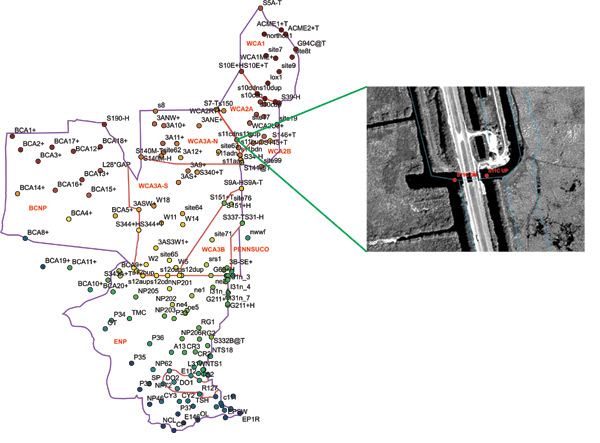
The initial EDEN study area consists of the freshwater domain of the Greater Everglades module extent with 206 water level gages that provided historical data for October 1999 through September 2004. Approximately a third of these stages have head and tail readings. Hourly water level data for the historical period were compiled for all existing water level gages in the study area and converted in NAVD 1988 vertical datum. Because of potential skew of hourly water level data, daily median was tested for the initial water surface analysis. The EDEN study area is hydrologically divided by canals and levees in WCA1, WCA2 (A & B), WCA3 (A & B), Big Cypress NP, Pennsuco and Everglades NP. Stratification of data is not always realistic since some areas have too few water stations, or stations are too far apart, beyond the spatial correlation distance. Thus, for the full set of data we choose to test Inverse Distance Weighting (IDW), Radial Basis Functions (RBF), regularized spline and multiquadric and harmonic functions for three different days for wet, dry and average conditions: Sep. 30, 2004, March 15, 2003, and Feb. 08, 2004. Kriging was thought to be unsuitable for EDEN water level surfacing because the hydrological connection is interrupted by canals and levees in the EDEN area and data spatial correlation is extremely weak.

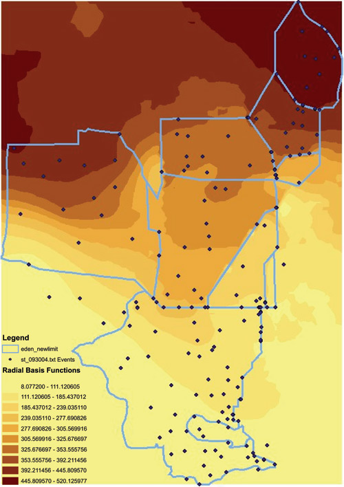
Generally speaking, RBF multiquadric negotiates border conditions along canals / levees better than IDW or completely regularize splines (CRS). RBF are a series of exact interpolation techniques (the interpolated surface honors the data points) that use a set of n basis functions, one for each location, while minimizing the total curvature of the surface (Johnston et al., 2003). The predictor is a linear combination of 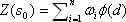where is a radial basis function with the Euclidian distance between the prediction location s₀ and each known data location s_i and the equation weights. The condition is that the radial basis function has to predict exactly the measured value when it is moved to the known data location.

The difference between a simple IDW and RBF interpolation is that IDW will have no predicted values below or above the minimum or maximum measured values, respectively. RBF predicted values, however, could be outside the measured values interval.

The multiquadric function is defined as: Equation where r is the smoothing or the shape parameter . If r is small the resulting interpolated surface has the minimal curvature forming a conelike basis function with the generated surface being very "tight" around the data points (Kansa and Carlson, 1992, Golberg et al., 1999, Johnston et al., 2003). As r increases the curvature of the function gradually flattens until the basis function is almost flat (Kansa and Carlson, 1992, Golberg et al., 1999). There is much discussion about how to choose the shape parameter r but no fool-proof method exist, only empirical formulas.

Comparison Between Kriging and RBF Multiquadric

Sirayanone (1988, cited in Hardy, 1990) has proved that the multiquadric method of interpolation generates a statistically unbiased result without being a stochastic method by setting the condition that the sum of the weight coefficients equals one. Hardy (1988) and Hardy and Sirayanone (1989) have proved that multiquadric and kriging methods have almost equal accuracy in bivariate distributions, multiquadric having the advantage to be easily transformed for stereo-viewing of 3D bodies, and does not require data stationarity as kriging does. Similar results regarding the equivalency of kriging and multiquadric interpolation results have been reported by Myers (1994) and Borga and Vizzaccaro (1997). Syed et al., (2003) using rainfall data,have demonstrated that multiquadric and kriging produce comparable results when variograms are developed using data from specific events, although kriging had inferior results when the variogram parameters were developed from monthly averages.

Discussion on EDEN Data

From all tested methods, IDW quadratic using a neighborhood with eight point data and RBF multiquadric with smoothing parameter equal with the minimum distance in-between data stations have given the best results. IDW has a smaller MSEP and average prediction bias than RBF multiquadric, while RBF multiquadric performs better regarding the variance of prediction error and the SE of the estimated mean bias. Visually, IDW produced less satisfying results because of a tendency to create "hills" surrounding data points.

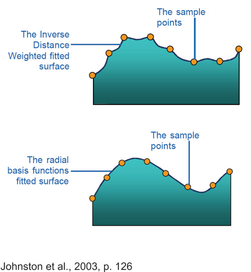
For each trial day we tested IDW and RBF regularized spline and multiquadric isotropic and anisotropic interpolations on the whole set of data, and on 12 different subsets corresponding to WCA1, WCA2A, WCA2B, WCA2 (A+B), WCA3A North (north of Alligator Alley), WCA3A South (south of Alligator Alley), WCA3A, WCA3B, WCA3 (A+B), WCA3+Pennsuco, Big Cypress NP and Everglades NP. Pennsuco and WCA2B areas have too few points to generate a geostatistical layer (mathematical graph of interpolation with continuous prediction surface). For WCA2B we could test only IDW interpolation to raster method, otherwise it was incorporated into WCA2 area. Overall RBF multiquadric had performed better than other methods negotiating better border conditions such as canals / levees. Further we tested only RBF multiquadric using isotropic and anisotropic search neighborhoods with standard or custom parameters. One of the custom parameters we always tested was equal with the minimum distance between the water stations used in interpolation. This parameter value is suggested by works of Gopfert (1977) and Hardy (1990).

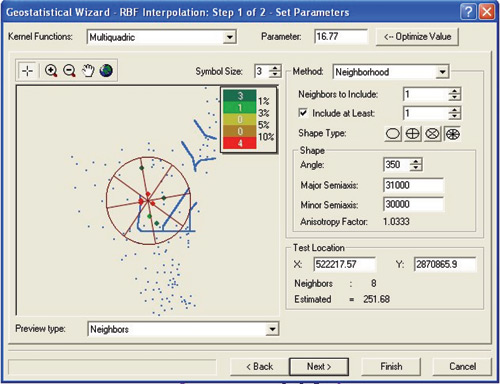
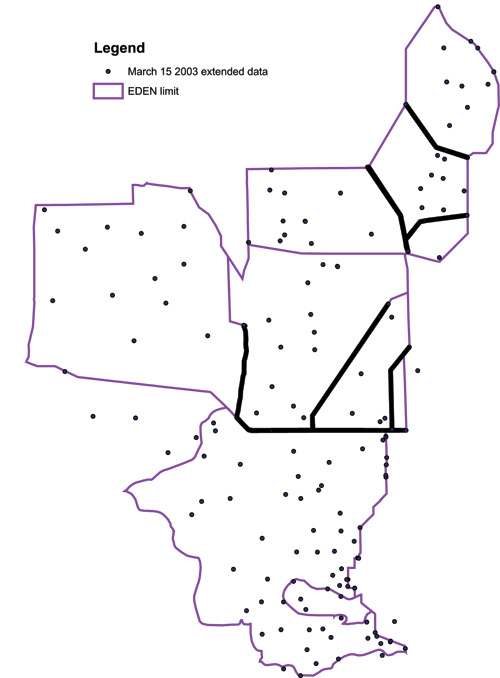
Overall RBF multiquadric performed the best when the shape parameter was equal with the minimum distance between two different water-gage stations. Since the canals / levees are hydrological barriers we tried to emulate those by linearly interpolating along those lines using head / tail stage data. These data were resampled every 200m and re-introduced into the interpolation exercise. Even if track data (preferential lines very densely sampled) alone may be problematic for interpolation, our mixture of track data along canals / levees, random distributed stage data and the provision to use only the closest data point to the interpolated location in each of the 8 sectors of search neighborhood may overcome some of the problems, but we will still have a reduced confidence in the interpolated surface close to canal data.

The N-S elongation of EDEN area suggests that an elliptical search neighborhood for interpolation might give better results. From all surfaces generated with the multiquadric method we selected 22 surfaces with 22 different sets of parameters that had small MPE and RMS errors and predicted maximum and minimum values not too far away from the maximum and minimum measured values. A set of parameters is composed of the r value, the angle of rotation for the search neighborhood and the two elliptical semi-axis. The search ellipse was divided in 8 sectors with equal angles of 45 degrees, and for each interpolated point we took into consideration one measured point in each sector that was closest to the center of the neighborhood ellipse. For each neighborhood ellipse we have tested several r parameters, including 0, optimal Franke, and minimum distance in between station locations. Through Geostatistical Analyst (ArcGIS 9.x,ESRI) we obtained a continuous mathematical representation of the water surface that further is sampled on a 400 x 400 m grid cell to record the predicted values.

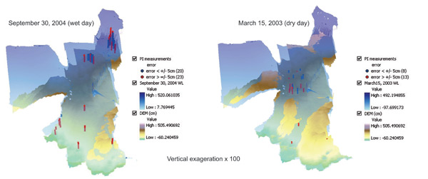
We evaluated calculated water depth surfaces using all 22 sets of interpolation parameters for representative wet, dry, and average days, and 4 different ground surface elevation interpolations (digital elevation models or DEMs). These water depths were compared with independently collected water depths data from other investigators (PI data). Differences between interpolated water depths and PI observed water depths may be due to the water surfacing algorithm, the DEM, water stage measurement error, PI measurement error, or fine terrain rugosity that is not captured on a 400m cell scale. The goal was to predict water depths to an accuracy of +/- 5 cm. Different methods performed slightly differently depending on which DEM we used. Some locations had differences greater than +/- 5 cm regardless of DEM or surface interpolation parameters used, while other locations seemed to be sensitive to the DEM used. In the figures below, it is apparent that differences between the predicted surface and PI observations of greater than +/- 5 cm occur clustered in the same areas as much smaller differences. This clustering of good and poor fits points towards elevation variability within the 400m grid cell as an important contributor to reported errors in predicted water depth. Future efforts will examine sub-grid cell depth responses, including the incorporation of proportion of vegetation community types as a variable in each cell.

Bibliography

Borga, M., and Vizzaccaro, A., 1997, On the interpolation of hydrologic variables, formal equivalence of multiquadric surface fitting and kriging, J of Hydrology no. 195, pp. 160-171

Gopfert, W., 1977, interpolationsergebnisse mit der multiquadratischen Methode, ZfV Z. VermessWes. 102, pp. 457 460, with summary in English

Hardy, R., 1988, Concepts and results of mapping in three dimensional space, Technical Papers, vol. 2, pp. 106 115, Cartography Am. Congr. Survey. & Mapp. 48th A. Meet., St. Luis, Miss.

Hardy, R., 1990, Theory and applications of the multiquadric-biharmonic method, 20 years of Discovery, 1968 1988, Comp. math Applic. Vol 19, no. 8/9, pp. 163 208

Hardy, R., and Sirayanone, S., 1989, The multiquadric-biharmonic method of three dimentional mapping inside ore deposits, Proc. 1989 Multinat. Conf. Mine Planning and Design, Univ. of Kentucky, Lexington, KY

Johnston, K., Ver Hoef, J. M., Krivoruchko, K., Lucas, N., 2003, Using ArcGIS geostatistical Analyst, ESRI

Myers, D.E., 1994, Spatial interpolation: an overview, Geoderma, vol. 62, pp. 17 - 28

Sirayanone, S., 1988, Comparative studies of kriging, multiquadric-biharmonic, and other methods for solving mineral resource problems, PhD. Disertation, Dept. of Earth Sciences,Iowa State University, Ames, Iowa

Syed, K.H., Goodrich, D.C., Myers, D.E., Sorooshiah, S., 2003, Spatial characteristics of thunderstorm rainfall fields and their relation to runoff, J. of Hydrology no. 271, p. 1-21

Citation

Palaseanu-Lovejoy, Monica, Ikuko Fujisaki, Leonard Pearlstine and Frank Mazzotti. (2006, June). Surfacing Daily Everglades Water Depths. Poster presented at the Greater Everglades Ecosystem Restoration Conference, Orlando, Florida.

The Croc Docs